Excel line chart with target range
Target chart and show the target value as a line in Excel. First of all let me show you the data which I am using to create a target line in the chart.
Create Dynamic Target Line In Excel Bar Chart
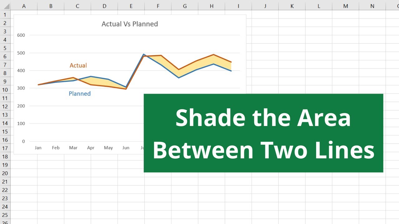
Create an actual vs.

. Select the data range and click Insert Insert Column or Bar Chart Clustered ColumnSee screenshot. 6In the Change Chart Type dialog box please specify the chart type of the new data series as Scatter with Straight Line uncheck the Secondary Axis option and click the OK buttonSee screenshot. The first step is to make your data table.
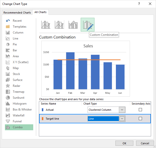
Instead of a formula enter your target values in the last column and insert the Clustered Column - Line combo chart as shown in this example. In my example I added 50 but if you are working with larger. Excel for Windows uses 1900 and Excel for Macintosh uses 1904.
Add a suitable chart title. Following dialog box will appear. Min 8 PM 083333 Max 10 AM 1416667 and Major Unit 2 hours 008333.
Get 247 customer support help when you place a homework help service order with us. I hope you found this tip. Surface Charts in Excel.
Follow these steps to shade the area below the curved line. There are several other ways to create a Target Vs. You can also change the color of your bars by your choice.
Here I have data on site visits of the week in the excel table. However Excel on either platform will convert automatically between one system and the. Radar Chart in Excel.
Now the task is to. This is used to cover the vertical lines of the target bars in the column chart. Add a cushion to the formula so that none of your target lines are at the very top of the chart.
This will align the line with the heads of target series. Select the range of data go to the insert tab click on column chart click on 2D chart. Click the line once to select it go to design tab click add chart elements hover above data labels click left.
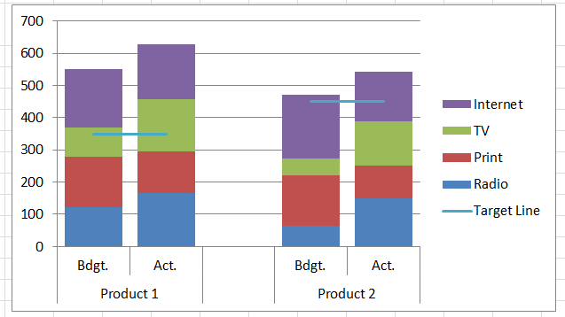
If the target value series is the second series in the chart in this step you need to right click at the Target Value series. Enter 2500 under major units and select thousands next to Display units. Learn how to create an actual vs budget or target chart in Excel that displays variance on a clustered column or bar chart graph.
Take the same table data. The primary axis displays the target and. In the inserted chart right click at the Actual Value seriesthen in the context menu click Format Data Series.
You can make it even more interesting if you select one of the line series then select UpDown Bars from the Plus icon next to the chart in Excel 2013 or the Chart Tools Layout tab in 20072010. Comparing to generally adding data series and changing chart type to add a normal horizontal line in a chart in Excel Kutools for Excels Add Line to Chart feature provides a fantastically simple way to add an average line a target benchmark or base line to a chart quickly with only several click. This table must have three main attributes Minimum Maximum and Range.
The epoch can be either 1900 or 1904. Chartwithtargetrangezip 14kb 30-Oct-13 CH0007 - Show Sparklines for Hidden Data -- Macro changes all sparklines on the active sheet so they will show data even if rows and columns are hidden. You can further format the above chart by making it more interactive by changing the Chart Styles adding suitable Axis Titles Chart Title Data.
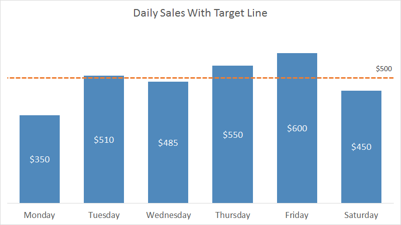
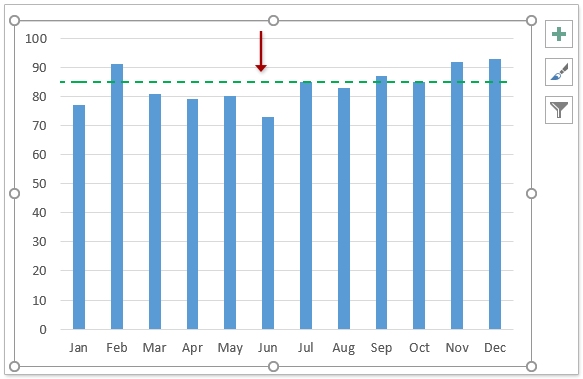
Excel stores dates as real numbers where the integer part stores the number of days since the epoch and the fractional part stores the percentage of the day. This section is going to show you how to create an actual vs. The horizontal line may reference some target value or limit and adding the horizontal line makes it easy to see where values are above and below this reference value.
Select line with markers under chart type for variance. A vertical line appears in your Excel bar chart and you just need to add a few finishing touches to make it look right. Now right-click target bar and select Change Series Chart Type.
5Now the benchmark line series is added to the chart. Plot in a line chart. You can change the courses using the drop-down list and the chart will.
Adding a target line or benchmark line in your graph is even simpler. Whirlpool Refrigerator Led Lights Flashing. You can use this formula and apply it to all corresponding cells.
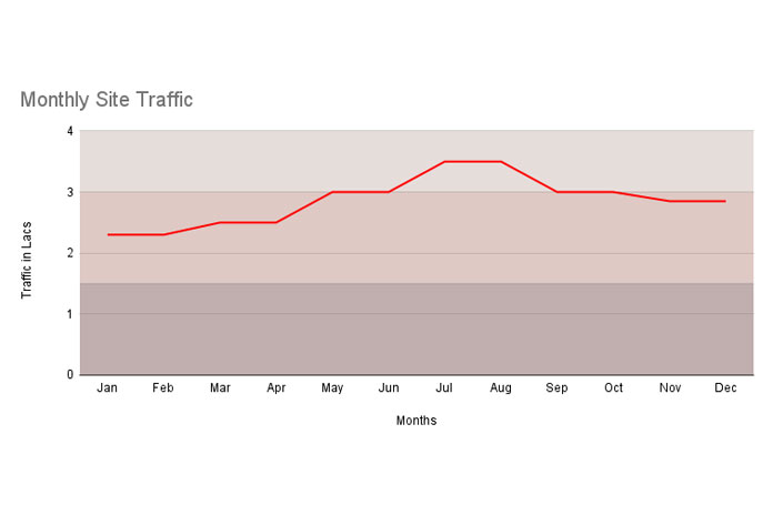
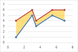
CH0008 - Show Target Range on Line Chart -- Show sales quantity in a line chart with target range shown in the background. Having the line still selected go to format tab click shape outline click no outline to hide the line. To the left of the top chart copy the range select the chart and use Paste Special to add the data to the.
We will guide you on how to place your essay help proofreading and editing your draft fixing the grammar spelling or formatting of your paper easily and cheaply. We have inserted a line chart using this data which looks something like this. You have a super quick method to copy chart formatting to another excel chart.
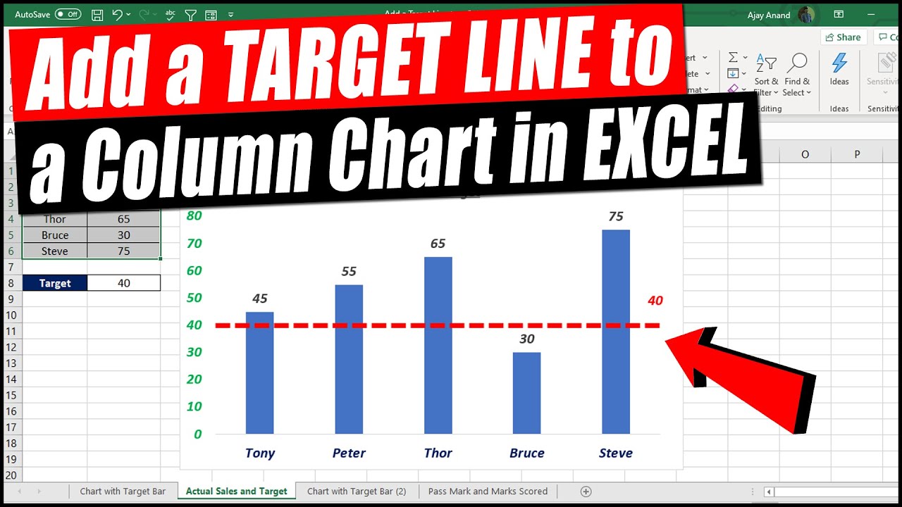
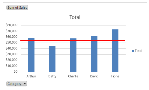
The Dynamic Chart is now ready to use. Following chart will appear showing target and actual values separately. To add the reference line in the chart you need to return the average of sales amount.
Select OK now right click on the Primary axis and select Format Axis. This is one more method which I often use in my charts is adding a target line. Free Excel file download.
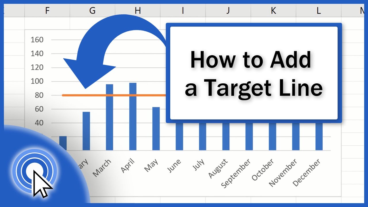
Add a Horizontal Target Line in Column Chart. Right-click the benchmark line series and select Change Series Chart Type from the context menu. It is the Value From Cells option in the Label.
Double-click the secondary vertical axis or right-click it and choose Format Axis from the context menu. Target values as bars. Now you can format the Trendline by selecting and clicking on the Format Trendline optionA dialog box will open where you can change the type and color of the trendline and also show the value in the chart.
I set the Y axis scale as follows. Now you dont have to worry about formatting multiple charts. 3D Scatter Plot in Excel.
You can also go through our other suggested articles Checklist in Excel. If none of the predefined combo charts. Only several clicks to add a line to a normal chart in Excel.
Here the range is the difference between the Maximum and the Minimum values. Follow the below steps to create a Tolerance chart in Excel. After inserting the chart two contextual tabs will appearnamely Design and Format.
If you will try to apply formatting from one chart for example bar chart to some other type of chart for example line chart it will also change the type of target chart. This will insert the labels for target series. Target chart and display the target values as lines as the below screenshot shown.
If you are using Excel 2013 there is a new feature that allows you to display data labels based on a range of cells that you select. After switching to LEDs or when replacing a faulty LED lamp in some cases the LED light will start flickering We will explain temperature settings alarm sounds door not closing water filter changes not cooling issues not making ice no power strange sounds leveling ice makers water dispensers This refrigerator has the. Add a shaded area under the line curve to the Excel Chart.
In this column a simple formula using the MAX function returns the largest value in your data range. Right click one of the horizontal grid lines and select delete. The same technique can be used to plot a median For this use the MEDIAN function instead of AVERAGE.
Create a Shaded Line Chart for Site Visit. From the Design tab choosethe Chart Style. Achievement chart but target line method is simple effective.
Select the data set created in step 9 and go to Insert followed by Chart Groups and insert a suitable chart. In the Format Axis pane under Axis Options type 1 in the Maximum bound box so that out vertical line extends all the way to the top. Now go to chart type of Target and select Line with Markers.
This is a guide to Excel Animation Chart. A common task is to add a horizontal line to an Excel chart. Here we discuss how to create excel animation chart along with practical examples and a downloadable excel template.
How To Add A Target Line To A Column Chart 2 Methods Youtube

Create Dynamic Target Line In Excel Bar Chart
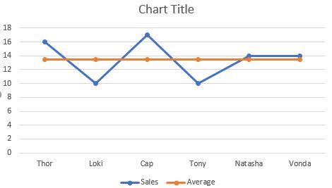
Highlight Above And Below Average In Excel Line Chart
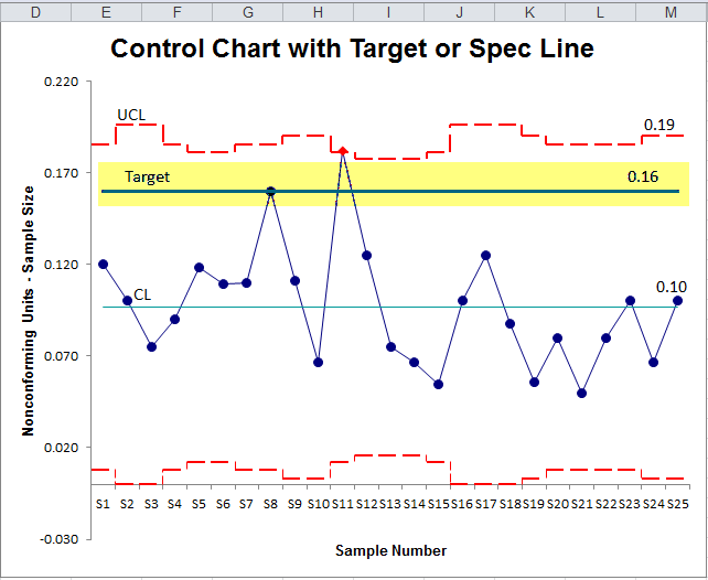
Add Target Line Or Spec Limits To A Control Chart
How To Add A Line In Excel Graph Average Line Benchmark Etc

How To Add A Horizontal Line To A Chart In Excel Target Average
How To Add A Target Line In An Excel Graph Youtube
3 Ways To Add A Target Line To An Excel Pivot Chart

How To Add Horizontal Benchmark Target Base Line In An Excel Chart
How To Add Horizontal Benchmark Target Base Line In An Excel Chart
Create A Shaded Target Range In A Line Chart In Google Sheets
Fill Under Or Between Series In An Excel Xy Chart Peltier Tech
How To Add Lines In An Excel Clustered Stacked Column Chart Excel Dashboard Templates
Line Graph With A Target Range In Excel Youtube
Combo Chart Column Chart With Target Line Exceljet
How To Add Horizontal Benchmark Target Base Line In An Excel Chart
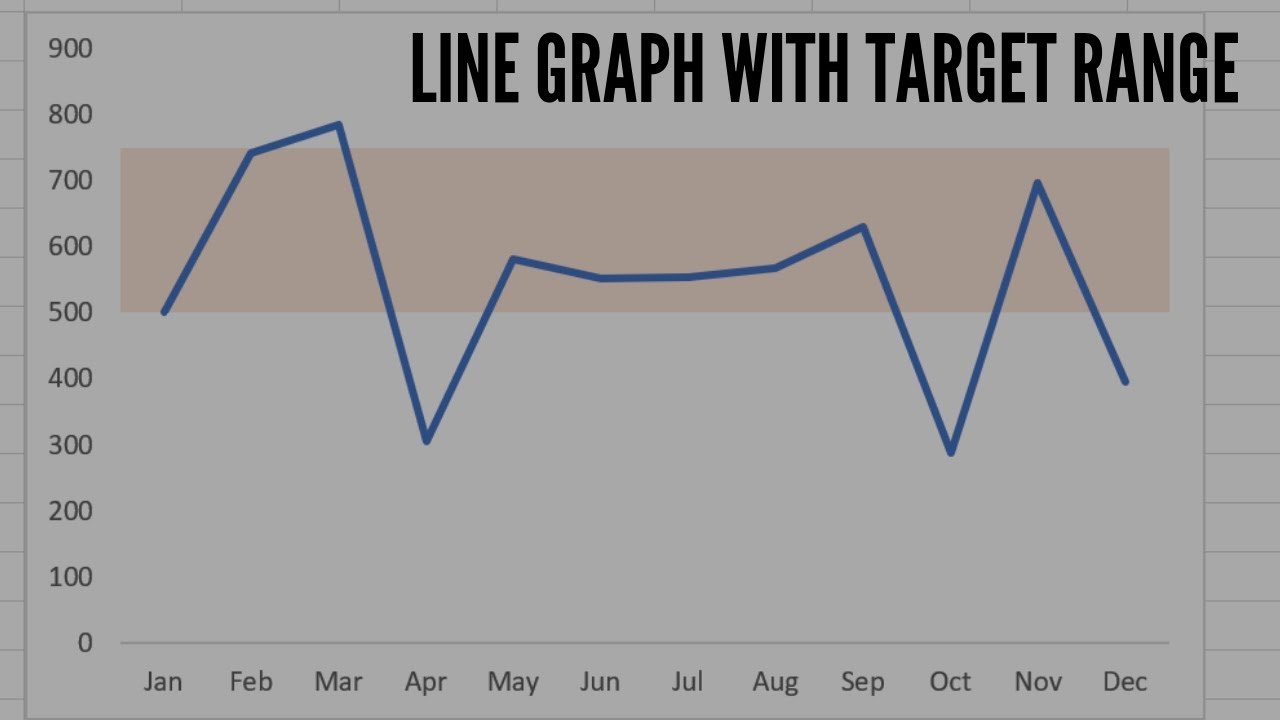
Line Graph With A Target Range In Excel Youtube